A new version of the Collatz Calculator is about to be released to the Apple App Store. The changes are somewhat experimental since they do not behave in a manner I would prefer but I wanted to get the functionality out for others to play with. If you are not familiar with the original version it is documented here. It is also important to be familiar with a design principal of the caclulator, that it will work across any Mx+B linear equation with both (M, B) pairs that work much the same way as 3n +1, that is (M, B) pairing that is what I call a member of the Colldilocks Set. This provides a means to study the effects of changing the (M, B) values and determine the behavior of individual sequences so that you can see which starting numbers will ultimately reach the value 1, and in the cases where the (M,B) pair is not a member of the Colldilocks Set, which numbers will result in an infinite loop or an infinite expansion.When using a non-Colldilocks pair, the graphml file will show the loopbacks, but knows when to stop when it encoulters an infinite expansion (Hint: No resolvable sequence will ever exceed n^3 *M. This way you can easily see which pairs produce a fully connected directed graph for the Colldilock pairs, and the broken sequences for the non-Colldilock pairs.
The latest version of the calculator introduces a memory as well as the capability of producing a graphml compliant file that can be used to graph the Collatz sequences. The memory is simply the collation of generated sequences. It is much more complicated to use at present, since all it does is take the current memory, generate the graphml description, and copy the result to the paste buffer. So to take advantage of this you would have to open your favorite text editor (Pages?), start a new document, paste the contents of the paste buffer into this new file, and export it as a plain text file and save it to the filesystem. At this point you would have to change the .txt extention to a .graphml extension. Once this is done, you can load it into any graphml viewing software such as the desktop application yEd from YWorks or even use their yEdLive website. I probably should mention that I receive no compensation from YWorks, that I don’t know and have not communicated with any of their employees, but am a long time user of their free version of yEd. So just to make sure I am clear, I have received no compensation of any type from YWorks, and they have received no money from me. But I love their application and am a very satisfied non-paying customer.
I probably should apologize for the Ta-Da effects. Even though you were able to disable this yourself through the app settings, I have decided that apps should be told to do things, but not heard unless something really really really needs to be communicated.
Let me know if this sounds intriguing, and feel free to send comments and or requests. I should mention that I also have the intent to release a windows version that will do arbitrary precision integers so that you can use virtually unlimited length integers, but constrained by the limits of the computer. Hey, even 32GB RAM is finite. Interested?
I have been working on a computational number model for a couple of years now, it has given me some insights including those that led to the Colldilocks set. I call it PSpace, a model where only primes exist. I won’t go into the details here, but suggest that besides the Colldilocks Set, I have discovered a new approach to searching for prime numbers.
When we talk about numbers, we have some very concrete terms that help us understand the nature of the Natural Numbers. The Natural Numbers are the positive integers, and probably gave us the first practical application of number theory which is captured in the concept of cardinality. When we left the world of the hunter/gatherer and began to pursue agriculture and domestication of animals for help in fulfilling our basic need for food, we needed an abstract means by which we could measure and control production. In short, we left the world of one, the one next meal, the one next hunt for fruits, vegetables, and protein to meet caloric needs. When we began to produce, rather than hunt, we produced surplus. And surplus needed to be managed. Now, instead of hunting for one animal, we had to manage a flock and a field of produce. To manage a flock or baskets of grain, fruits, and vegetables we needed to know how many. How many cattle. How many sheep.
We needed to handle addition and subtraction to handle the herd replenishments by births or outside acquisition, and the losses by consumption or predation. Through time, we became more complex in our number theory through qualitative concepts such as Ordinality. We began to recognize the aspects of even and odd numbers, powers like squares and cubes, and basic aspects like prime and composite. Concepts grow and change. We changed our means of counting from notches on a stick, to knots on a rope, to stylus impressions on clay, and finally to glyphs on paper. Roman numerals gave way to numerical digits. We have standardized on the base ten number systems so that our representation of a magnitude could be grasped within the human mind as a series of the sums of products. The number 437 for instance is understood to be a shorthand for 4 * 100 + 3 * ten + 7 * 1. We created number systems as tally shortcuts for the cognitive limitations of our own brains. But suppose we would like to know how a number is factored. It may be easy to understand that 4 is 2 * 2, and 53 is a prime with only 1 and 53 as factors. But what about 40437121?
Factoring very large numbers is very hard and is the foundation of all internet security. The security of Public Key Infrastructure is based on this fact that allows me to publish my public key with no fear that my private key can be calculated because my public key is so large that a computer cannot factor it in reasonable time. But what if we could create a numerical model based on a dimensional space representing only the products of primes that could be searched via some heuristics that could map any given magnitude to its location in the space? This is one of my investigations. My world is PSpace which is a directed graph of nodes with three edge types. Diversity is the edge that manifests numerical difference. Purity is the edge that manifests numerical purity. Finally, Harmony is the edge that produces numerical hybridization. I will reserve further elaboration of this model to a future posting, but for now I can introduce a second discovery based on this model.
What follows is a python program that utilizes this conceptual model to generate the PSpace and produce the list of primes between one and N. It varies from our current sieve models, whether we use Eratosthenes, Sundaram, Atkins, or a wheel sieve, in that it only requires a single iterative loop for whatever value you choose for N. The sieve algorithms require multiple iterative loops, at least one for marking the truthfulness of primality for the current iteration’s magnitude, and then a final iteration to traverse the sieve to reap the primes. In the generation of the PSpace, we not only discover the prime numbers, but also record the factorization of all nodes within PSpace.
PSpacePrimes.py
#
#   Author:        Derwin Charles Skipp
#   Created Date:  16-Mar-2021
#   Description:   This program will generate primes using the PSpace hanging vector method
#
import math
import string
import sys

#   Program Globals

limit = int(pow(2, 20))        # set 1M as default limit
PSpace = {}
totalCalculations = 0
totalDiversityNonprime = 0
totalDiversityPrime = 1        # Must count 2 as the first prime
totalPurity = 0
totalHarmony = 0


# Hanging vectors for prime search

diversityHangingVector = {}
purityHangingVector = {}
harmonyHangingVector = {}

# Primes list

primesList = []

#
#   I like printf
#
def printf(format, *values):
    print(format % values, flush=True)

#
#
#
def prompt(prompt):
    print(prompt +": ", end='', flush=True),
    response = str(sys.stdin.readline())
    return response.rstrip()

#
#    Construct and populate a new PSpace node
#
def newNode(magnitude, parent, diversity, purity, harmony, dbase, dtail, ptail, htail):
    thisNode = {}
    thisNode["magnitude"] = magnitude
    thisNode["parent"] = parent
    thisNode["diversity"] = diversity
    thisNode["purity"] = purity
    thisNode["harmony"] = harmony
    thisNode["dbase"] = dbase
    thisNode["dtail"] = dtail
    thisNode["ptail"] = ptail
    thisNode["htail"] = htail
    return thisNode


##############################################################
#                                                            #
#   Generate the PSpace sequentially using hanging vectors   #
#                                                            #
##############################################################

#   This is the heart of the single threaded sequential generation of the PSpace
#   It is a search to find thisNode's parent node and set the proper vector
#   to point to this new but not yet connected PSpace node.
#   It will either be the last determined prime's uncalculated vector and thus a new prime,
#   or match a precalculated hanging vector.
#   There are two options:
#   if magnitude matches a hangingVector, a calculated magnitude vector for an existing
#       PSpace node that does not have a corresponding PSpace node
#       update parent node hangingVector to thisNode and remove from hangingVector dictionary
#       calculate each hangingVector for thisNode and add them to hangingVector dictionary
#       populate thisNode's remaining attributes
#   else we found a prime!
#       set parentNode to lastPrime
#       insert this magnitude into primesList
#       set last found prime node to thisNode's parent and set diversityVector to thisNode
#       calculate parentNodes harmonyVector hangingVector for thisNode and add it to the hangingVector dictionary
#       populate thisNode's remaining attributes

#
#   createPSpaceNode
#
def createPSpaceNode(magnitude):
    global PSpace
    global totalCalculations
    global totalDiversityNonprime
    global totalDiversityPrime
    global totalPurity
    global totalHarmony
    global diversityHangingVector
    global purityHangingVector
    global harmonyHangingVector
    #   Note, since the probabilities of a node being a diversity,
    #   purity, harmony, or primary diversity (prime) occur with
    #   rising probabilities, they are tested for in that order;
    #   however, since primes occur with more frequency in a
    #   magnitude bound pspace, they still have to wait until
    #   all hanging vectors are checked.

    #   If this magnitude in the diversity hanging vector, we found a diversity node
    if magnitude in diversityHangingVector:
        #   We found a diversity composite
        totalDiversityNonprime += 1
        #
        #   update parent node hangingVector to thisNode and remove from hangingVector dictionary
        #
        parentMagnitude = diversityHangingVector[magnitude]
        parentNode = PSpace[parentMagnitude]
        del diversityHangingVector[magnitude]
        #
        #   calculate each hangingVector for this Node and add them to hangingVector dict
        #
        dbase = parentNode["dbase"]
        dtail = parentNode["dtail"] +1
        ptail = parentNode["ptail"] +1
        htail = parentNode["htail"] +1
        diversity = dbase * primesList[dtail]
        #
        #   since we are creating a magnitude bound PSpace, do not create a PSpace node > limit
        #
        if diversity <= limit:
            diversityHangingVector[diversity] = magnitude
        else:
            return
        purity    = magnitude * primesList[ptail]
        if purity <= limit:
            purityHangingVector[purity] = magnitude
        harmony   = magnitude * primesList[htail]
        if harmony <= limit:
            harmonyHangingVector[harmony] = magnitude
        #   Add 3 for diversity, purity, and harmony to total calculations
        totalCalculations += 3
        #   create thisNode and add it to PSpace
        thisNode = newNode(magnitude, parentMagnitude, diversity, purity, harmony, dbase, dtail, ptail, htail)
        PSpace[magnitude] = thisNode

    #   If this magnitude in the purity hanging vector, we found a purity node
    elif magnitude in purityHangingVector:
        #   We found a purity composite
        totalPurity += 1
        #
        #   update parent node hangingVector to thisNode and remove from hangingVector dict
        #
        parentMagnitude = purityHangingVector[magnitude]
        parentNode =PSpace[parentMagnitude]
        del purityHangingVector[magnitude]
        #   calculate each hangingVector for thisNode and add them to hangingVector dicts
        diversity = "";   # There is no diversity vector on a purity node!
        dbase = magnitude
        dtail = parentNode["dtail"]
        ptail = parentNode["ptail"]
        htail = ptail +1
        purity = magnitude * primesList[ptail]
        if purity <= limit:
            purityHangingVector[purity] = magnitude
        harmony = magnitude * primesList[htail]
        if harmony <= limit:
            harmonyHangingVector[harmony] = magnitude
        #   Add 2 for purity and harmony to total calculations
        totalCalculations += 2
        #   create thisNode and add it to PSpace
        thisNode = newNode(magnitude, parentMagnitude, diversity, purity, harmony, dbase, dtail, ptail, htail)
        PSpace[magnitude] = thisNode

    #   If this magnitude in the harmony hanging vector, we found a harmony node
    elif magnitude in harmonyHangingVector:
        totalHarmony += 1
        #   Get parent node
        parentMagnitude = harmonyHangingVector[magnitude]
        parentNode = PSpace[parentMagnitude]
        del harmonyHangingVector[magnitude]
        #
        #   calculate each hangingVector for thisNode and add them to hangingVector dict
        #
        dbase = parentNode["magnitude"]
        ptail = parentNode["htail"]
        htail = parentNode["htail"] +1
        dtail = htail
        diversity = dbase * primesList[dtail]
        diversityHangingVector[diversity] = magnitude
        purity  = magnitude * primesList[ptail]
        if purity <= limit:
            purityHangingVector[purity] = magnitude
        harmony = magnitude * primesList[htail]
        if harmony <= limit:
            harmonyHangingVector[harmony] = magnitude
        #   Add 3 for diversity, purity, and harmony to total calculations
        totalCalculations += 3
        #   create thisNode and add it to PSpace
        thisNode = newNode(magnitude, parentMagnitude, diversity, purity, harmony, dbase, dtail, ptail, htail)
        PSpace[magnitude] = thisNode
        #   Delete the completed parent PSpace node since it is no longer necessary for future calculations
        # del PSpace[parentMagnitude]
    #  PSpace conjecture 1: If this magnitude is not in a hanging vector then we found a prime!
    else:
        totalDiversityPrime += 1
        printf("%d", magnitude)
        #   get parentNode which will be the last prime magnitude
        lastPrimePtr = len(primesList) - 1
        lastPrime = primesList[lastPrimePtr]
        parentNode = PSpace[lastPrime]
        parentMagnitude = parentNode["magnitude"]
        #   insert this magnitude into primesList
        primesList.append(magnitude)
        #   set parent's diversity vector to thisNode's magnitude
        parentNode["diversity"] = magnitude
        #
        #   calculate parentNode's hanging harmonyVector and add to the harmonyHangingVector dict
        #
        parentHarmony = parentMagnitude * magnitude
        if parentHarmony <= limit:
            #
            #   now you can update the parent prime PSpace node with updated vectors
            #
            parentNode["harmony"] = parentHarmony
            harmonyHangingVector[parentHarmony] = parentMagnitude
        #
        #   calculate this node's hanging purity vector and add it to the hangingPurity dict
        #
        dbase     = magnitude
        dtail     = parentNode["dtail"] +1
        ptail     = parentNode["ptail"] +1
        htail     = parentNode["htail"] +1
        purity = magnitude * magnitude
        if purity < limit:
            purityHangingVector[purity] = magnitude
        #  Add 2 for purity, and parent harmony to total calculations
        totalCalculations += 2
        #   create thisNode and add it to PSpace
        thisNode = newNode(magnitude, parentMagnitude, "", purity, "", dbase, dtail, ptail, htail) # diversity & harmony are Unknown at this point
        PSpace[magnitude] = thisNode

#   findPSpacePrimes
#   Generate the root and first primary diversity node, and search for the next magnitude's location in the PSpace
#   with Node Magnitude, Node Type, Node Parent, Diversity, Purity, Harmony, DBase, dtail , pTail, and hTail
def findPSpacePrimes():
    #   prime the PSpace with the non prime and non composite anomalous root node of magnitude 1
    #   Note: The axiomatic declaration of 2 as the first prime is a programatic optimization to prevent the need
    #   to add a conditional check for first prime found within the createPSpaceNode() found prime code
    #   This way we do not have to make the determination of the root node update vs the prior prime node update
    #   But really, the determination of the primality of 2 would be found since all hanging vectors would be empty
    #   The root node with magnitude 1 is anomylous as the only PSpace node with undefined purity and harmony vectors
    #   The first prime node with magnitude 2 is anomylous as the only PSpace diversity node with an even magnitude
    #   All other PSpace nodes behave themselves with purity nodes lacking a defined diversity vector
    #   Call me, we can discuss.
    thisNode = newNode(1, "", 2, -1, -1, 1, 1, 1, 1)
    PSpace[1] = thisNode
    thisNode = newNode(2, 1, -1, 4, -1, 2, 0, 0, 1);
    PSpace[2] = thisNode
    printf("2")
    #   prime the primesList
    primesList.append(2)
    #    prime the purity hanging vector with 2^2
    purityHangingVector[4] = 2
    #    Generate the rest of PSpace up to defined limit
    for magnitude in range(3, limit+1):
        createPSpaceNode(magnitude)

###############################
#                             #
#   P R O G R A M   M A I N   #
#                             #
###############################

if (len(sys.argv) - 1) > 0:
    limit = int(sys.argv[1])
else:
    limit = 1000000
findPSpacePrimes()
print("Total calculations: {}    There are {} primes between 1 and {}".format(totalCalculations, len(primesList), limit ))
print("Total Diversity: nonprime {}   prime {}   Total Purity: {}   Total Harmony: {}".format(totalDiversityNonprime, totalDiversityPrime, totalPurity, totalHarmony))
print("Total Nodes {}".format(totalDiversityNonprime + totalDiversityPrime + totalPurity + totalHarmony + 1))
Please, let me know your thoughts about this PSpace prime search.
Update: 2022/05/30 PSpacePrimes.py updated to remove horrific bug producing erroneous prime list.
Admitting my rather recent introduction and study of the Collatz Conjecture I have been perplexed by the problem definition that is different from the one that I presented in my last posting titled “Collatz and The Three Bears”. I have heard various mathematicians present a conceptional problem definition that does not complete but rather, in the 3n + 1 problem, closes upon the 4 -> 2 -> 1 -> 4 … infinite loop. This is an heresy from the computational perspective since it is difficult to solve a generalized problem that by definition does not end with a final, or accepting state. Given that the formal definition of a finite state automata (FSA) or Turing machine is defined to be:
That is to say that there needs to be a set F which is a subset of the finite, non-empty set of states Q that defines a final or accepting state. Thus, in my previous posting step two of the 3n + 1 algorithm is to halt if the computed value is equal to one.
There are two very different approaches to mathematics. In 1973, a mathematical conference was held jointly by the American Mathematical Society and the Mathematical Association of America, and titled the “Conference on the Influence of Computing on Mathematical Research and Education”. It was here that Peter Henrici of Swiss Federal Institute of Technology Zürich (Eidgenössische Technische Hochschule or ETH) coined the terms “algorithmic mathematics” and “dialectic mathematics”. And this distinction as quoted directly from Peter Henrici’s paper was:
“Dialectic mathematics is a rigorously logical science, where statements are either true or false, and where objects with specified properties either do or do not exist. Algorithmic mathematics is a tool for solving problems. Here we are concerned not only with the existence of a mathematical object, but also with the credentials of its existence. Dialectic mathematics is an intellectual game played according to rules about which there is a high degree of consensus. The rules of the game of algorithmic mathematics may vary according to the urgency of the problem on hand.”
We are most familiar with mathematics of the dialectic sort. But surprisingly, algorithmic mathematics does not require a computer. In fact, one of the earliest examples of algorithmic mathematics is from a Babylonian clay tablet from the 18th century BC that defines an algorithm for approximating the square root of 2. The steps are simple:
Step 1: Try and guess the square root of 2.
Step 2: Divide your original number by your guess.
Step 3: Find the average of your guess and the result of step 2.
Step 4: if the difference of the guessed number and the average is close enough then stop, otherwise go to step 2 using the average as your next guess.
To this day we have no function f(n) = Pn where Pn is the nth prime. The sequence of prime numbers are found through one of many sieve algorithms from Eratosthenes through Atkins or a wheel sieve, which themselves are examples of algorithmic mathematics. Do we then propose that an Algorithmic approach will not be able to produce a proof of the conjecture since it is by nature outside of the dialectic world of true/false? Remember Bertrand Russell and Alfred Whitehead’s Principia Mathematica? Or can an algorithmic approach lead to insights that will allow for a Dialectic proof? What if we do not attempt to provide a dialectic proposition of truth or falsehood, but rather focus on a computational model that will allow us to perceive insight leading to understanding how something works.
I approach this problem algorithmically using a computation model of the Natural Numbers, and consequently would like to introduce the product of my efforts and the first offering from Sophwares – The Collatz Calculator. I am curious as to the interest in such an application. At present, I have a version for IOS targeted to an iPhone or iPad, and a version for MacOS for the Apple Mac computer that soon, I hope, will be available from the Apple App Store.
Interested?
Here are some screen shots.
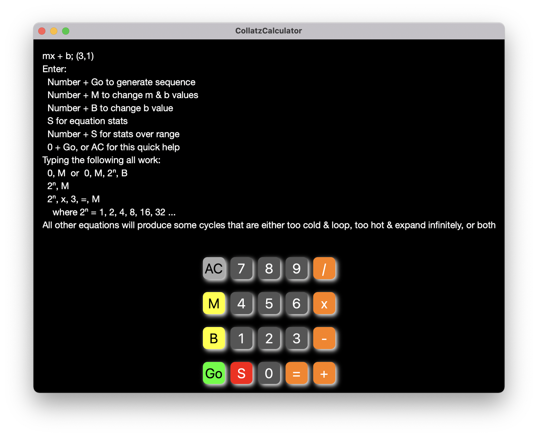
When you start the application you will see the quick help screen:
When you type 27 and Go you will see the sequence generated for 27:
When you type S, you will see the stats for n = 1 to 100:
Since the conjecture suggests that the sequence generated for any value of n will resolve to one for 3x + 1, it becomes more interesting when you change the formula. This is accomplished with the M and B buttons. The M button will allow you to set the M value and calculates a value for b based on whether M is the first value of a Colldilocks pair (M, B). If M = 0, B will be set to 2. If M is a power of 2, then B will be set to the same power of 2, and if M = 3 times a power of 2, B will be set to the power of 2. Otherwise, M will be set to any value that is not the first value of a Colldilocks set pair and B will be set to 1. B will be set to whatever value you type as a number, and press the B button.
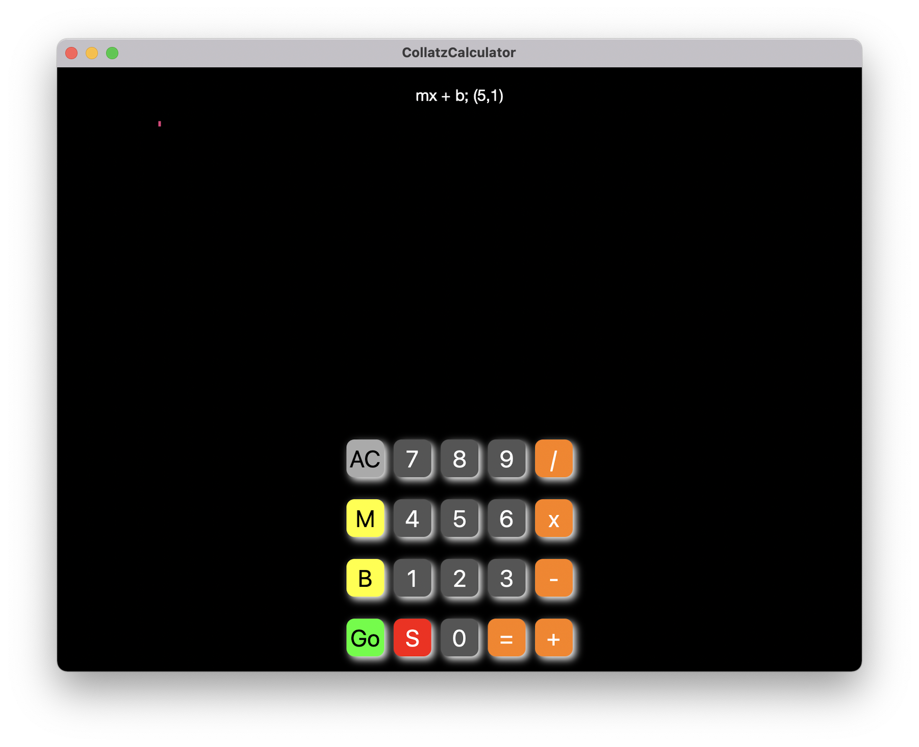
When you type 5, M you will see the (M,B) pair set to (5, 1):
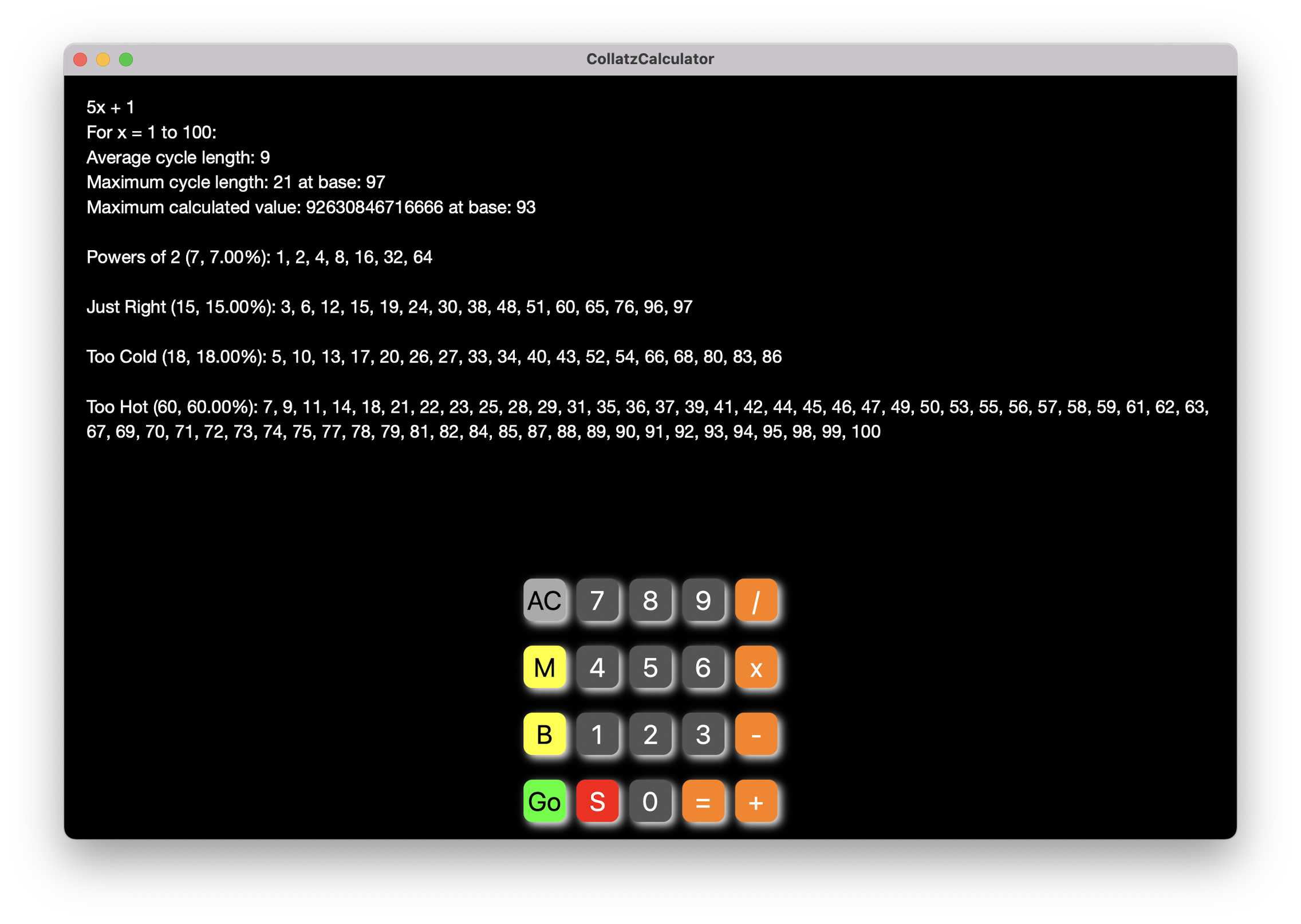
When you type S, you will see the stats for n = 1 to 100 for 5x + 1:
The stats page indicates the formula under consideration. It will show the range of x, which can be set by first typing the maximum value for x (default 100). But be careful here, especially on a iPad or iPhone. The larger the range, the busier your calculation since it has to generate all sequences for all x between 1 and N. It also reports the average cycle length (excluding the infinite too hot, and too cold cycles). It will report the maximum cycle length over the range and the first value for x that generates a cycle of that length. It will also show the highest calculated value over the range and the first value for x that reaches that peak. In cases where the x value is too cold and loops, it will show you at which step the number repeats and the index of the first occurrence of the repeating value. And if the value of x is too hot, it will predict when it believes that the values will simply continue an upward trend towards infinity. It will also present lists of x values that are powers of 2, and if applicable, the list of x values that will resolve to 1 (just right), the list of x values that will produce a loop (too cold), and the list of x values that it predicts will lead to infinite expansion (too hot). If you type one of the values of x displayed on the stats page it will display the cycle for that value.
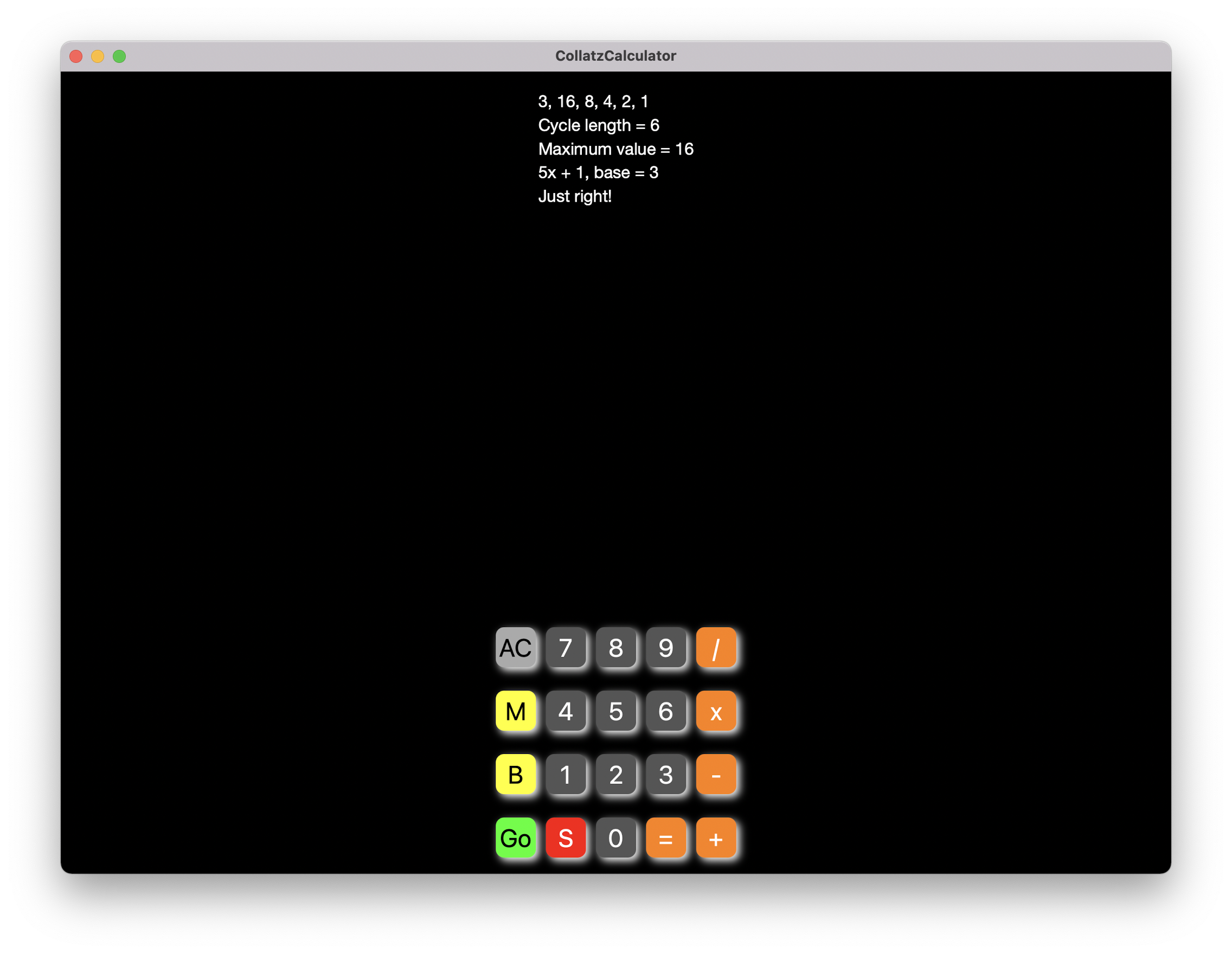
Now when you type 3 and Go you will see the “just right” sequence generated for x = 3 when y = 5x +1:
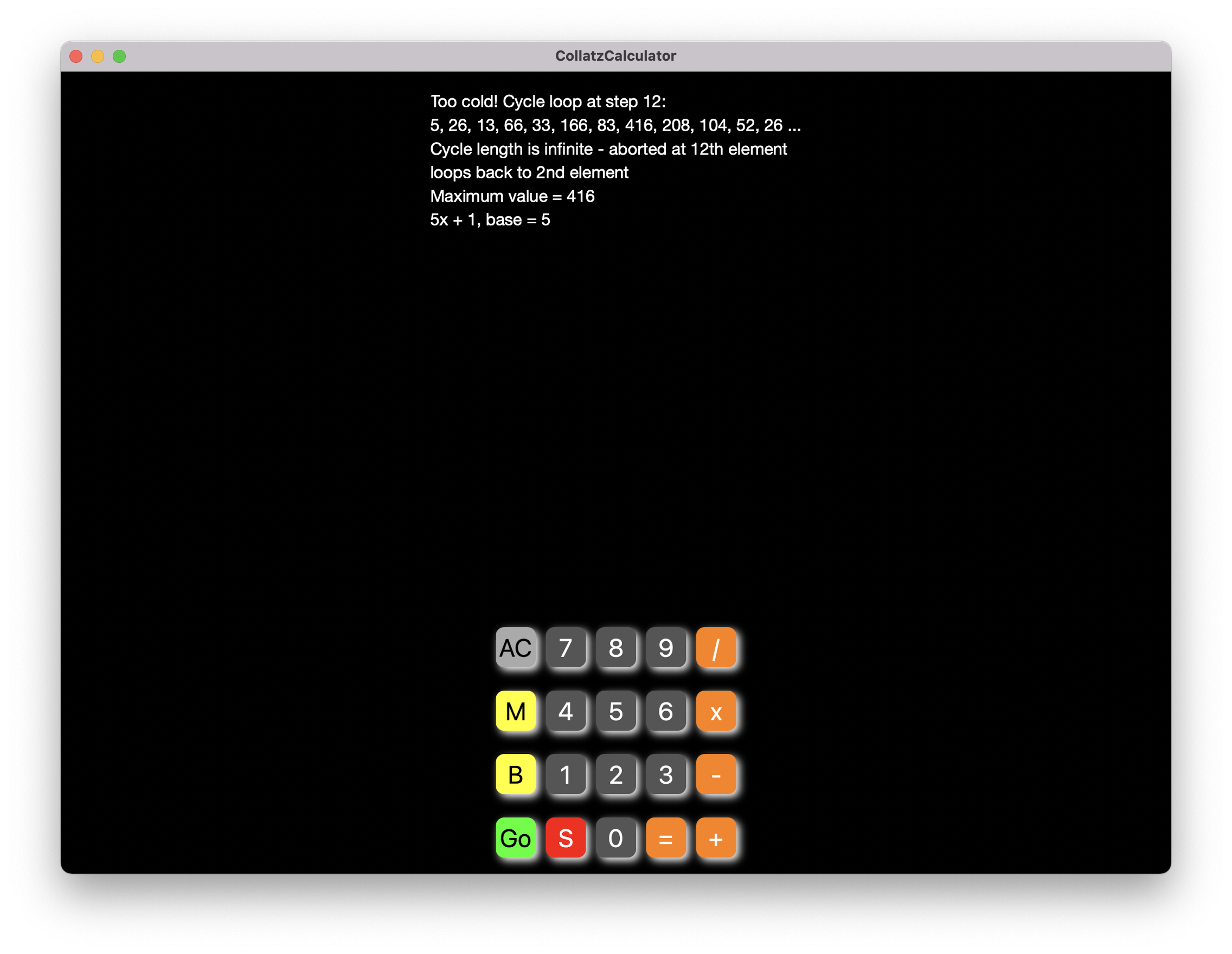
If you type 5 and Go you will see the “too cold” sequence generated for x = 5 when y = 5x +1:
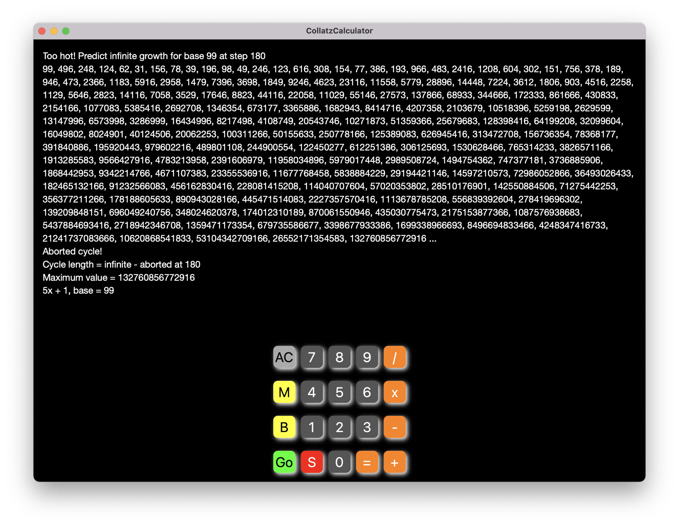
And if you type 99 and Go you will see the “too hot” sequence generated for x = 99 when y = 5x +1:
The Collatz Calculator will allow you to study the Collatz Conjecture across any value of the generalized linear equation y = mx + b for all values of m, x, and b.
Lothar Collatz was a German mathematician born on the 6th of July, 1910. In 1937 he proposed a rather simple yet mind boggling problem that has since come to be known as the Collatz Conjecture. It is now recognized as a classic unsolved mathematical challenge, and a great enigma. The problem, also known as the 3x +1 problem is actually very easy to explain. It is the rather simple algorithm as follows:
Step 1: Start with any positive natural number. Step 2: If the number is 1, stop. Step 3: If the number is even, then divide it by 2, else it is odd, then multiply it by 3 and add 1. Step 4: Go to step 2 with the resulting number.
It appears that, regardless of the starting number, the sequence of numbers produced by following these simple steps will always close on the following sequence: 16-8-4-2-1. More importantly, it will always lead to the value 1, which means according to step 2, we will always halt the sequence generation and more importantly, this will occur for all values of x. The problem and intriguing aspect of the conjecture is that since its inception, nobody has been able to prove that it is true for all cases of x regardless of how big we make it.
This is not to say that we haven’t tried. The current record for the count of numbers tested stands at 2 raised to the 68th power. For those less familiar with powers of 2, that would be 295,147,905,179,352,825,856. That’s a very large number, but even though all numbers in this range do lead to sequences that end in 1, it is not a proof for all values of x.
So let us take a walk with this problem by suggesting a comparison to the well-known children’s tale of Goldilocks and the Three Bears. I will not repeat the story except to point out the introduction of the theme of too hot, too cold, and just right, and the need for a slight restatement of the problem.
The 3x +1 problem is a simple case of that class of mathematical expressions that we call a linear equation. And linear equations are rather important within mathematics. The 3x+1 equation is in a specific form that we call the slope-intercept form and generalize it to be:
y = mx + b Where m is a constant that defines the slope of the line b is a constant that reflects the y-intercept point of a plot on an XY graph And x is the variable that y is dependent upon
So what is it about m = 3 and b = 1 that gives us this magical consistency in resolving all generated sequences to the value 1 when using this equation in the above 4 step algorithm? It is important to note that when m is not 3 and b is not 1, it is quite possible and actually more likely that you find some cycles will not ever stop at step two and generate a sequence of numbers for some values of x that go on for ever. And it is here that we make the connection to the children’s tale. Since for all values of x, you will produce a sequence of numbers. The exception case is when x is chosen to be 1 and you will end with a single value. Otherwise, in the terminology of the problem we produce a sequence of numbers ending in 1 that we call a cycle. Examples would be if we start with the number 3 then we would get the sequence:
3 -> 10 -> 5 -> 16 -> 8 -> 4 -> 2 -> 1
But the cycle lengths can be big. For instance if we chose to start with 27 we get:
In fact, we don’t seem to have a limit as to how big a cycle can be, we just guess that they will all eventually end at the value 1 for 3x + 1.
But we do know that if we try other values for m and b, we can get cycles that never end. And they will not end in one of two ways. They will either repeat a value that has already been encountered within the current cycle, in which case the sequence will repeat in an infinite loop. Or we will get an unlimited growth in the value of the result of the odd number cases. For instance, if we choose m = 3 and b = 2, it is probably very clear that the sequence will be infinite since for any odd number multiplied by 3 followed by the addition of 2 will always be odd.
3 -> 11 -> 35-> 107 -> 323 -> 971 … for ever in a 3x +2 expansion!
If we choose m = 3 and b = 3 This will be an infinite loop between step 2 and 3. And if we chose 3 for m and 3 for b we get:
We also know that we can chose some values that result in behavior identical to the 3x + 1, which is to say that we will always generate a sequence that ends at the value 1 regardless of our chosen value for the variable x.
In the simplest case take the value 0 for m and 1 for b. We get the following sequences:
And so on. In this case we can prove that the sequence will always end at the value 1 since, if x is even, we keep dividing it by 2 until it is either odd or 1. And if x is odd, it will always become 1 since (0 * x) + 1 will always equal 1 regardless of the value of x.
In fact there are an infinite number of Collatz Conjecture like number pairs for (m, b) that will behave as the 3x + 1 problem. Most values for any arbitrary chosen pairs will result in infinite sequences by either looping on a repeating sequence (too cold) or an infinite expansions of ever increasing calculations on odd numbers (too hot).
But it turns out that some pairs are just right and result in all sequences for any given value for n will converge on the value 1. The only variables are the lengths of the cycle, the convergent values between two different sequences, and the point of convergence onto the closing sequence of powers of 2 that ultimately resolve to 1.
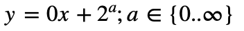
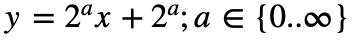
The existence of this set of number pairs that behave the same as the 3x + 1 problem with all sequences generated for all values of n that converge on 1 will be called the Colldilocks set. The Colldilocks set can be calculated by the union of the sets of the m and b pairs of the following 3 formulas:
All m,b pairs will always have some values of n that will be just right and resolve to one. The choice of any power of 2 will never exit the even expression and will always resolve to one by constant division by 2. Some m,b pairs may have some values of n that also resolve to 1. However, any m,b pair outside the Colldilocks set will fail with at least some cycles generated for some values of n that will be too hot or too cold leading to the following conjecture:
Conjecture: All (m,b) pairs within the Colldilocks set will generate cycles that resolve to 1 for all values of x. All (m,b) pairs that are not in the Colldilocks set will result in some values of x that produce cycles that will be either too hot or too cold with the possibility that some non power of two values for x will produce cycles that will resolve to 1.
Welcome to SophWares, a destination that I humbly suggest as, and hope to develop into, a new model for the educational information economy. SophWares is more about a journey for us all as we live, grow, and learn. Especially focused on teaching and learning, SophWares aims to contribute to the educational environment, both through the formal channels of educational institutions K-12, higher education and upward, as well as the private and solo endeavors of the “forever student”. SophWares aims to become a site for collaborative effort that will address fundamental questions of value and a hope for new ideas to help build a foundation for a fair and just marketplace, with secure information exhange, and with reasoned compensation for creative effort.
I am concerned that educational institutes have lost their way as thought leaders and contributors to the advancement of information technology, both within the confines of the educational information infrastructure as well as the explosion of the internet outside of academia and research into the social and commercial IT systems of today. Particularly, we have failed miserably in providing for a secure foundation with which to exchange private information for self-edification and commerce as reflected in the continuous revelation of information breaches. It is my hope to address this issue here by revisiting the foundations of secure communication involving both trustworthy authentication and fine grained access controls.
I am concerned that our educational systems are not reaching the full potential of the promises of the computer-enriched learning environment. I have recently retired from one of the largest universities in the country. I wonder if you, like me, find that educational institutions have stumbled a bit by focusing effort on classroom enrichment through computer as medium rather than the revolution that could be with the computer as simulated reality. We have replaced the age-old professor with lecture behind the lectern and presenting on the white or black board with podcasts of professors with lecture behind the lectern displaying on the white or blackboard and sometimes enhanced with a Powerpoint presentation.
SophWares is committed to simple principals. The first is that the educational experience is revolutionary when the mediated classroom is enhanced with computer simulation. When the student is challenged by the “what if” scenarios driven by personal interaction with a well-developed simulation, then the student moves on from the memory storage device to the companion thinking entity brimming with understanding. I would like to present within this forum some examples of challenging simulations.